The following is a basic and jargon-free explanation of how it is possible to detect causal relationships in molecular networks and between molecules and phenotypes. If you are new to biological networks, for broad reviews of the origin of molecular networks and their relationships to disease please see reviews by Barabasi and Csermely . To quickly see large molecular networks surrounding the molecules you're interested in, try Genemania . In contrast, our results are focused on the regulatory structure active around individual genes and their relationships to Alzheimer’s disease phenotypes.
How can we tell if a gene is upstream in a signaling cascade or upstream of a phenotype? We use “causal inference” methods that are applied to combinations of omics data, which have all been measured in the same set of people. The mathematical basis of this work goes back to conditional independence and Bayesian inference, but in this tutorial we focus on their simple practical application.
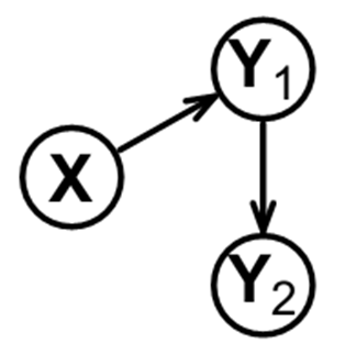
Let’s start with a simple case wherein you measure data from three variables. These variables are typically molecules, whose levels you can measure in multiple samples or people, who we consider to be snapshots of the same regulatory system at different state-times. Let’s call these three variables: X, Y1 and Y2. Let’s say that the true biological regulation among these variables is as shown below, where X regulates Y1, and then Y1 regulates Y2, as shown below.

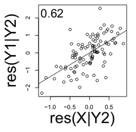
This is the sort of information we wish to learn in the future, just from looking at raw data, when the true regulation is unknown. To uncover the true relationship among these three variables, simply from data generated by this system, consider what happens when you “condition” expression of one variable on another variable. The notation for this is X|Y, meaning the residual levels of X after Y has been regressed out. If consider the relationship of X and Y1, (below) when they are both conditioned on Y2 (i.e. Y1|Y2 and X|Y2), note that there remains a relationship between X and Y1.
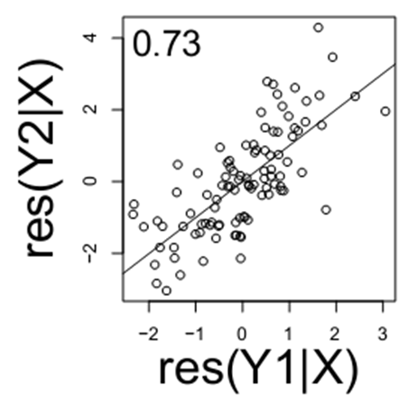
Similarly, if you look the relationship of Y1 and Y2 (below), note there is still a relationship when conditioning on the variable X (below).
However, if you account for Y1, note the relationship between X and Y2 is lost (below).
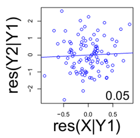
This indicates the likely relationship among these three variables is a chain between X, Y1 and Y2 with no direct link between X and Y2. The examination of these various residuals is an example of how we begin to transition from mere replicate data (typically expression levels) to directed networks among variables in the dataset.
Now let’s examine a different network structure among the variables and the data it generates. In this instance, X causally affects both Y1 and Y2 (below).
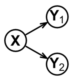
This network structure (above) is different than the previous example, wherein a chain of activation led from X to Y1 to Y2. From our observations about the previous example, you can guess that conditioning on X in the network shown above will reduce the Y1-Y2 relationship. You can also guess that no other variable (Y1 or Y2) will have such an effect (as demonstrated below).

Going back to our first example of data from X1→Y1→Y2, there is a tricky point we’ve omitted thus far. The pattern of data below….

is equally compatible with X → Y1 → Y2 and X ← Y1 ← Y2 (notice how the regulation is running in opposite directions). In both of these possible networks, we have ruled out a link between X and Y2, but how do we tell which way the arrows should be oriented? The way we can tell which way the arrows should be oriented is through a biological fact: genetics are largely unchanging while gene expression is flexible. At least in a non-cancer state, the genome typically does not change in response to gene expression, but gene expression can be increased or decreased by genetic polymorphisms. These genetic variants that results in gene expression changes as called eQTL’s. If “X” in our network is an genetic locus that drives gene expression, then we can conclude the correct model is X → Y1 → Y2, because regulation from Y1 → X would violate the biological principle of genetics regulating gene expression.
You can apply the logic of causal inference to large collections of variables by taking them three at a time and applying the type of causal inference shown above. After you apply it to one set of three nodes, you can move on to define other parts of the network. Here’s an example of applying causal inference to small groups of nodes, iteratively, to generate a large network. This one happens to be composed of microglia-related genes.
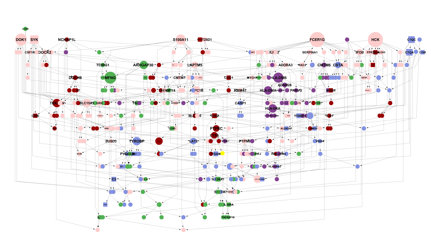
In theory inferring the structure of large networks involves more of the same process used to define networks of three nodes. However, in practice computational and statistical challenges limit the accuracy of large network reconstruction. For instance, a network comprised of 100 variable-nodes can form a number of possible network structures that exceeds the number of atoms in the observable universe (~1078). For such large networks, the accuracy of the inferred structure improves when you refine it strategically, avoiding getting “stuck” in a bad solution. You can try out the top-performing methods described in this paper that can effectively refine the structure of big networks. For networks with only several nodes, like those produced for this site, the number of possible network states is not very large (though still in the millions) so the network structures are likely close(r) to the global optimum.
Thanks to Elias Chaibub Neto for the graphics on this page.